Graphical Method Linear Programming

Linear programming problems with two decision variables can be easily solved by graphical method. A problem of three dimensions can also be solved by this method, but their graphical solution becomes complicated.

Basic Terminology - Graphical Method

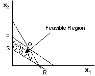
Feasible Region

It is the collection of all feasible solutions. In the following figure, the shaded area represents the feasible region.

Convex Set

A region or a set R is convex, if for any two points on the set R, the segment connecting those points lies entirely in R. In other words, it is a collection of points such that for any two points on the set, the line joining the points belongs to the set. In the following figure, the line joining P and Q belongs entirely in R.

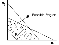
Thus, the collection of feasible solutions in a linear programming problem form a convex set.

Redundant Constraint

It is a constraint that does not affect the feasible region.

Example: Consider the linear programming problem:

Maximize 1170 x₁ + 1110x₂

subject to

9x₁ + 5x₂ ≥ 500
7x₁ + 9x₂ ≥ 300
5x₁ + 3x₂ ≤ 1500
7x₁ + 9x₂ ≤ 1900
2x₁ + 4x₂ ≤ 1000

x₁, x₂ ≥ 0

The feasible region is indicated in the following figure:

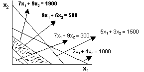
The critical region has been formed by the two constraints.

9x₁ + 5x₂ ≥ 500
7x₁ + 9x₂ ≤ 1900

x₁, x₂ ≥ 0

The remaining three constraints are not affecting the feasible region in any manner. Such constraints are called redundant constraints.

Extreme Point

Extreme points are referred to as vertices or corner points. In the following figure, P, Q, R and S are extreme points.